Statistics
The
Poisson Distribution

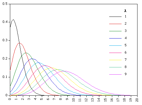
In the picture above are simultaneously portrayed several Poisson distributions. Where the rate of occurrence of some event, r (in this chart called lambda or l) is small, the range of likely possibilities will lie near the zero line. Meaning that when the rate r is small, zero is a very likely number to get. As the rate becomes higher (as the occurrence of the thing we are watching becomes commoner), the center of the curve moves toward the right, and eventually, somewhere around r = 7, zero occurrences actually become unlikely. This is how the Poisson world looks graphically. All of it is intuitively obvious. Now we will back up a little and begin over, with you and your mailbox.
Suppose you typically get 4 pieces of mail per day. That becomes your expectation, but there will be a certain spread: sometimes a little more, sometimes a little less, once in a while nothing at all. Given only the average rate, for a certain period of observation (pieces of mail per day, phonecalls per hour, whatever), and assuming that the process, or mix of processes, that produce the event flow are essentially random, the Poisson Distribution will tell you how likely it is that you will get 3, or 5, or 11, or any other number, during one period of observation. That is, it predicts the degree of spread around a known average rate of occurrence. (The average or likeliest actual occurrence is the hump on each of the Poisson curves shown above). For small values of p, the Poisson Distribution can simulate the Binomial Distribution (the pattern of Heads and Tails in coin tosses), and it is much easier to compute.
The Poisson distribution applies when: (1) the event is something that can be counted in whole numbers; (2) occurrences are independent, so that one occurrence neither diminishes nor increases the chance of another; (3) the average frequency of occurrence for the time period in question is known; and (4) it is possible to count how many events have occurred, such as the number of times a firefly lights up in my garden in a given 5 seconds, some evening, but meaningless to ask how many such events have not occurred. This last point sums up the contrast with the Binomial situation, where the probability of each of two mutually exclusive events (p and q) is known. The Poisson Distribution, so to speak, is the Binomial Distribution Without Q. In those circumstances, and they are surprisingly common, the Poisson Distribution gives the expected frequency profile for events. It may be used in reverse, to test whether a given data set was generated by a random process. If the data fit the Poisson Expectation closely, then there is no strong reason to believe that something other than random occurrence is at work. On the other hand, if the data are lumpy, we look for what might be causing the lump.
The Poisson situation is most often invoked for rare events, and it is only with rare events that it can successfully mimic the Binomial Distribution (for larger values of p, the Normal Distribution gives a better approximation to the Binomial). But the Poisson rate may actually be any number. The real contrast is that the Poisson Distribution is asymmetrical: given a rate r = 3, the range of variation ends with zero on one side (you will never find "minus one" letter in your mailbox), but is unlimited on the other side (if the label machine gets stuck, you may find yourself some Tuesday with 4,573 copies of some magazine spilling all over your front yard - it's not likely, but you can't call it impossible). The Poisson Distribution, as a data set or as the corresponding curve, is always skewed toward the right, but it is inhibited by the Zero occurrence barrier on the left. The degree of skew diminishes as r becomes larger, and at some point the Poisson Distribution becomes, to the eye, about as symmetrical as the Normal Distribution. But much though it may come to resemble the Normal Distribution, to the eye of the person who is looking at a graph for, say, r = 35, the Poisson is really coming from a different kind of world event.
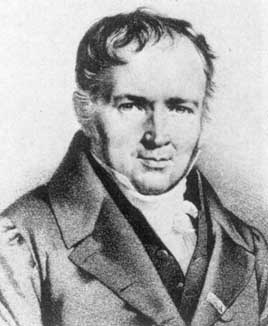
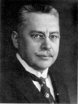
History. The Poisson Distribution is named for its discoverer, who first applied it to the deliberations of juries; in that form it did not attract wide attention. More suggestive was Poisson's application to the science of artillery. The distribution was later and independently discovered by von Bortkiewicz, Rutherford, and Gosset. It was von Bortkiewicz who called it The Law of Small Numbers, but as noted above, though it has a special usefulness at the small end of the range, a Poisson Distribution may also be computed for larger r. The fundamental trait of the Poisson is its asymmetry, and this trait it preserves at any value of r.
Derivation. The Poisson Distribution has a close connection with the Binomial, Hypergeometric, and Exponential Distributions, and can be derived as an extreme case of any of them. The Poisson can also be derived from first principles, which involve the growth constant e. That derivation is given on a separate page, for those who like to see the inner workings of the universe up close. Other readers may proceed directly to the how-to-do-it instructions in the next section.
Computing Poisson Probabilities
We found, on the Derivation page, that when the average rate of occurrence of some event per module of observation is r, we can calculate the probability of any given number of actually observed occurrences, k, by substituting in the formula
Before going on, consider the following:
It will be noticed that in our formula, the only variable quantity is the rate r. That number is the only way in which one Poisson situation differs from another, and it is the only determining variable (parameter) of the Poisson equation. Nothing else enters in.
Each number r defines a different Poisson distribution. We cannot multiply by 10 the values for the distribution whose rate is r = 1 and get the values for r = 10. The latter must be calculated separately, and will be found to have a different shape. Specifically, the larger the r for any given unit of occurrence, the more symmetrical is the resulting frequency profile. This we already noticed in the picture at the top of this page.
What we here call rate of occurrence, or r, is conventionally called lambda (l). Remember to make that adjustment when consulting other textbooks or tables.
Calculating Poisson probabilities ideally requires a statistical calculator, with x*y and e*x keys (remember that e is the constant 2.71828). Absent such a calculator, certain individual probabilities may be computed with the aid of the e*x Table. For selected simple values of r, problems may be solved using the Tables here provided.
Example. Let us suppose that some event, say the arrival of a weird particle from outer space at a counter on some farm outside Topeka, occurs on average 2 times per hour. But there are variations from that average. What is the probability that in a given hour three weird particles will be recorded? Substituting in formula (5) the empirical rate r = 2 and the expectation k = 3, we get:
p(3) = r*3 / 3!e*r = 2*3 / 6e*2 = 8 / (6)(7.3891) = 8 / 44.3346 = 0.1804
This answer may be checked with the one given in the Poisson Table, and will be found to match. This sort of calculation was in fact how the Table was constructed.
In rough terms, then, if our weird particles average 2 per hour but vary randomly around that average, and thus fit the random Poisson model, we would expect to get 3 rather than 2 weird particles per hour, at the counter over by the silo, in about 0.1804 of the hours observed. If we only watch for one hour, our reading will most likely be 2 particles. But there are 24 hours in a day, and in an average day, there should thus be (24)(0.1804) = approximately 4 hours during which 3 particles are registered. Of course, things can vary from that most likely expectation; that is the way the universe works. But now we know what the most likely expectation is. It is such likeliest expectations that the Poisson formula gives us.
Just to show how the whole situation looks, here, from the Table, is the frequency profile for r = 2, omitting the extremely rare possibilities:
p(0) p(1) p(2) p(3) p(4) p(5) p(6) p(7) p(8) p(9)
It will be seen that the realistic possibilities for occurrence per hour go no lower than zero (which would be physically impossible), and that they reach as high as 9 per hour before becoming so miniscule that they do not show up in four decimal places. If we add these probabilities, we get 0.9999, or 1 (the total probability in the system) plus an effect of rounding error. This, then, is a virtually complete picture of the possibilities. So also with every other column of the Table.
Browsing one of those Tables will illustrate the fact that the Poisson is cramped on the zero side, but spreads out on the infinity side. The list of possible values is thus asymmetrical (the statistical term is "skew"). Such situations, where variation from an average is easier in one direction than another, are very common in real life, and this is one thing that accounts for the fact that so many situations are well described by the Poisson distribution. (For the Normal Distribution, the assumption is that variation is equally likely in either direction from the average).
For the set of probabilities (frequency profiles) for selected average rates r, consult the Poisson Table. To calculate individual probabilities, use formula (5) above. Rough probabilities may be obtained by the use of Poisson Paper. This, and clear thinking, are all that are required to work with the Poisson distribution. The clear thinking is the hardest part, as the Problem set will presently demonstrate.
The Classic Example
The classic Poisson example is the data set of von Bortkiewicz (1898), for the chance of a Prussian cavalryman being killed by the kick of a horse. Ten army corps were observed over 20 years, giving a total of 200 observations of one corps for a one year period. The period or module of observation is thus one year. The total deaths from horse kicks were 122, and the average number of deaths per year per corps was thus 122/200 = 0.61. This is a rate of less than 1. It is also obvious that it is meaningless to ask how many times per year a cavalryman was not killed by the kick of a horse. In any given year, we expect to observe, well, not exactly 0.61 deaths in one corps (that is not possible; deaths occur in modules of 1), but sometimes none, sometimes one, occasionally two, perhaps once in a while three, and (we might intuitively expect) very rarely any more. Here, then, is the classic Poisson situation: a rare event, whose average rate is small, with observations made over many small intervals of time.
Let us see if our formula gives a close fit for the actual Prussian data, where r = 0.61 is the average number expected per year for the whole sample, and the successive terms of the Poisson formula are the successive probabilities. Remember that our formula for each term in the distribution is:
We may start by asking, given r = 0.61, what is the probability of no deaths by horse kick in a given year (module of observation)? For k = 0, we get by substitution
p(0) = (0.61)*0 / (0!)(e*0.61) = 1 / (1)(1.8404) = 0.5434
Given that probability, then over the 200 years observed we should expect to find a total of 108.68 = 109 years with zero deaths. It turns out that 109 is exactly the number of years in which the Prussian data recorded no deaths from horse kicks. The match between expected and actual values is not merely good, it is perfect.
If we had used instead, as an approximation, the value of e*0.6 from our table, we would have gotten p(0) = 0.5488, so that the expected number of such years over 200 years would be 109.76 = 110, or 1 too high. Not bad.
For the entire set of Prussian data, where p = the predicted Poisson frequency for a given number of deaths per year, E is the corresponding number of years in which that number of deaths is expected to occur in our 200 samples (that is, our p value times 200), and A is the actual number of years in which that many deaths were observed, we have:
and the match seems very good throughout. (Not perfect. But it is intuitively obvious that another trial, over another 200 years' worth of data, would give slightly different results, and this is a perfectly plausible example of one such result).
In sum, then, we assume that the Poisson frequency profile gives the expectation (E) when the events in question are indeed random. Comparing that expectation with our actual results (A), we judge that the Prussian data set appears to be the result of random causes. There is no reason to suspect any systematic cause, or any connection between separate events. These deaths, then, just happened. (If ill-trained horses were supplied to all corps in one year, for instance, the pattern of deaths should be more clustered, and we would have a nonrandom factor). It is the ability of the Poisson Distribution to give a model for stuff that "just happens," that accounts for its power in statistics. Statistics is about stuff that "just happens."
The Poisson distribution has several unique features. Most distinctively, as noted above, it has only one parameter, namely the average frequency of the event. That figure is conventionally called lambda (l); we here use instead the abbreviation r (for rate).
The Poisson distribution is not symmetrical; it is skewed toward the infinity end.
The mean of any Poisson distribution is equal to its variance, that is
m = v
which is a unique property of this distribution. (Note that "mean" here is the average of all values, and defines the center of gravity of the distribution; it is not a point from which values diverge symmetrically; the Poisson Distribution is not symmetrical). It is sometimes said that the Poisson mean is an "expectation." It is true that the commonest frequency in any Poisson set is the one corresponding to r itself. But it is also true that if r is a whole number, the expectation for (r-1) is identical to that for r, so that where r > 1, the "expectation" is a pair of outcomes, not one single outcome.
For fractional r, where the likeliest or equally likeliest frequency is 0, the histogram of a Poisson set of frequencies is high on the left and skewed toward the right. For the Prussian horse data, above, where r = 0.61, it looks like this:
As the average frequency (r) increases, the histogram becomes a little humpier in the middle (see the Poisson Table for an overview of the pattern up to r = 20), but it never becomes perfectly symmetrical, and thus it never loses its distinctive character as a distribution. That character, however, does weaken with increasing r.
Poisson paper is specially printed for the easy analysis of raw data. If you plot data points on Poisson paper, they will lie on a vertical line if the set is random in the sense assumed by the Poisson formula. If the resulting line is not vertical, then to that degree, the data set is non-Poisson.
The situations to which Poisson distributions apply are diverse, and it is not always easy to see at first glance that they are specimens of one underlying type. We give here examples of three common types of Poisson problem. These sample problems will be repeated on the Practice page, along with other problems of the same general type.
Keep in mind that all we have to work with are (1) a rate of occurrence, r, which may be any number; (2) a window of observation; a timespan or a space within which occurrences are observed, and (3) the number of times the event, as seen through that given window, is repeated.
Isolated Events
It has been observed that the average number of traffic accidents on the Hollywood Freeway between 7 and 8 PM on Wednesday mornings is 1 per hour. What is the chance that there will be 2 accidents on the Freeway, on some specified Wednesday morning?
Answer. The basic rate is r = 1 (in hour units), and our window is 1 hour. We wish to know the chance of observing 2 events in that window. The rate r = 1 is included in the Poisson Table, so we don't have to calculate anything. Reading down the r = 1 column, we come to the p(2) row, and there we find that the probability of 2 accidents is 0.1839, or a little less than 1 chance in 5. It's not unlikely. You might get that situation about once a week.
Proportions
Coliform bacteria are randomly distributed in a certain Arizona river at an average concentration of 1 per 20cc of water. If we draw from the river a test tube containing 10cc of water, what is the chance that the sample contains exactly 2 coliform bacteria?
Answer. Our window of observation is 10cc. If the concentration is 1 per 20cc, it is also 0.5 per 10cc; that is just another way of saying the same thing. So r = 0.5 is the rate relevant to our chosen window (if we used a 20cc test tube, or window, the rate would be different, and the resulting frequency profile would also be different). We can then read off any desired probability from the r = 0.5 column of the Poisson Table. For the specific value of p(2), the table supplies the answer 0.0758, or about 1 chance in 13. Not common, but not out of the question either. About once in 8 tries with that unit of observation.
Arrivals
The switchboard in a small Denver law office gets an average of 2.5 incoming phonecalls during the noon hour on Thursdays. Staffing is reduced accordingly; people are allowed to go out for lunch in rotation. Experience shows that the assigned levels are adequate to handle a high of 5 calls during that hour. What is the chance that 6 calls will be received in the noon hour, some particular Thursday, in which case the firm might miss an important call?
Answer. The rate 2.5, and the window of observation is 1 hour. The desired result is easily read off the Poisson Table, from the p(6) row of the r = 2.5 column. The answer is p(6) = 0.0278, or about 1 chance in 36, or a little more than 1 missed phonecall per month. How acceptable that is will depend on how cranky the firm's clients are, and the firm itself is in the best position to make that judgement.
Besides handling Poisson problems proper, the Poisson Distribution can give an useful simulation of the Binomial Distribution when p is small (one rule of thumb is that it should be no greater than 0.1). In these cases, q is known (as in true Poisson problems it is not), but it is simply discarded; we pay no attention to it. In the range where the Poisson approximation is reasonably close, it is much less difficult to calculate, and is often preferred in practice.
Sample Binomial Problem
Rick has a crooked quarter, which comes up Heads 80% of the time. He tells Jimmie he will get 7 or more Heads in 10 tosses. Jimmie bets the family horse that there will be 6 or fewer Heads. What is Jimmie's chance of riding home from the wager?
This can be worked out by Binomial methods, which are the ones strictly proper to it. To adjust to Poisson perspectives, we take as r the rate of the rarer event (T = Tails), with an average rate of 2 per 10 tosses or 0.2. This exceeds the above recommended level, but we will go ahead anyway, just to see what happens.
We are making a trial observation for another 10 tosses. The expectation for those 10 tosses is ten times the rate for one toss; hence we expect T = 2, and the rate also becomes 2 (per set of 10). Rick bet on between 3 and 0 Tails, so Jimmie wins only if the 10 tosses yield 4 or more Tails. From the Poisson Table for r = 2, we find that the sum of probabilities p(4) through p(9) gives 0.1428, or about 1 in 7, as Jimmie's chance of winning. (There is no value for p(10), that frequency being so small that it does not show up in four place decimals, so it is not included in the table).
If we go back and do this over as as a Binomial problem, we would have have n = 10 (there are 10 tosses), and p(T) = 0.2000 (the coin comes up Tails, on average, 2 times out of 10). The exact Binomial answer for Rickie's chance of winning (to four places) is 0.1209. The Poisson approximation was 0.1428. The Poisson approximation in this case is 18% high; that is, it is only roughly right. This is the consequence of our having exceeded the recommended figure of p = 0.1. This may remind us that Poisson is not an easier way of getting any and all Binomial results. It is a different animal, one which under certain conditions leaves similar tracks as it lopes on its own errands through the statistical woods.
- The Poisson distribution deals with mutually independent events, occurring at a known and constant rate r per unit (of time or space), and observed over a certain unit of time or space.
- The probability of k occurrences in that unit can be calculated from p(k) = r*k / (k!)(e*r).
- The rate r is the expected or most likely outcome (for whole number r greater than 1, the outcome corresponding to r-1 is equally likely).
- The frequency profile of Poisson outcomes for a given r is not symmetrical; it is skewed more or less toward the high end.
- For Binomial situations with p < 0.1 and reasonably many trials, the Poisson Distribution can acceptably mimic the Binomial Distribution, and is easier to calculate.
The first of these items is mandatory, for practice with the above Poisson explanation (you don't know it until you can do it). The second and third are problems dealing with the number e, which plays a fundamental role in questions of this type. The rest are a mix of Sinological and standard puzzlements, some of which have turned up elsewhere in this site, and are gathered here for their recreational value.
- Poisson Problems
- The King's Coiner
- Ozzie's Risk
- The Gwodyen Problem
- The Birthday Problem
- The Prisoner's Dilemma
Tables
- Factorials
- Poisson Table
- Extended Poisson Table
- Pascal Triangle
- Right Pascal Triangle
- Powers of e
- Fractional Powers of e
- Eric Temple Bell
- Jacob Bernoulli
- Abraham de Moivre
- Albert Einstein
- Carl Friedrich Gauss
- Boris Gnedenko
- William S Gosset
- Blaise Pascal
- Simeon-Denis Poisson
24 Aug 2007 / Contact The Project / Exit to Home Page
This and other Statistics pages are Copyright © 2005 by E Bruce Brooks, University of Massachusetts at Amherst


